
Byline: A brief overview of terms and considerations when conducting and reading a static analysis of permanent magnets.
When Quadrant perform magnetic circuit simulation, the acronym FEA is often brought up by our engineers. The FEA stands for Finite Element Analysis. It’s a common simulation method in many software packages for electro-magnetic fields, heat, and stress. It boils down to breaking a 2D or 3D representation of the environment into a series of nodes (or points) at which the quantity being simulated can be calculated. This usually requires breaking the model down with a meshing software, which creates the points (however many are needed or specified) in the program before the calculations are done.
Finite elements are just a way of saying that the calculations are done in a finite number of points representing the model, instead of simulating the model in a continuous fashion. We can then smooth the results between the points using linear interpolation. Hopefully, the mesh was fine enough that this still gives a valid answer. This is a large concern in FEA, a sensitivity analysis (seeing how the different variables affect your results and controlling the error) will need to be conducted to make sure the mesh is of a proper size to accurate portray the original system. This can take some time and experience.
Many EM (electro-magnetic) simulation packages break each point of the simulation down into a virtual coil and use Clark Maxwell’s equations for calculating electric and magnetic fields. This is simplified, of course, but essentially, that’s where we are start.
The goal of EM FEA is often one of two things in 95% of cases; to find the flux density in a specific area - perhaps to trigger a hall-effect sensor, or to find the magnetic force between objects. We should focus on those two separately, although they are inherently related. The simplest calculation for magnetic force between two objects is F = B2A/2μ0 (Cardarelli, “Materials Handbook”, 3rd edition, page 745, derivation of Maxell’s force equation). Which is the average flux density across an area between the objects multiplied by the area itself (this area is often whatever face is in contact while holding). The value ‘B’ refers to flux density (magnetic flux/area).
For a hall-effect sensor application, one would need to know, from the sensor manufacturer, at which flux density the sensor triggers on and at what value it is released (this is assuming a simple binary sensor, an analog sensor will give a varying voltage in a range). The simulation environment can then be created to match the real world as accurately as possible. The position of the permeant magnet in relation to the sensor is key. Many hall effect sensors will read in a single component direction of flux density (a single-axis sensor). Flux density is a vector, which means it has a direction and magnitude. If a single-axis sensor is used, it must be placed perpendicular to the component of the flux density that needs to be read. By default, the software will provide a flux density magnitude (|B|). The components will be known as Bx, By, and Bz in a cartesian coordinate system. These will be trig function values of the total magnitude, depending on their angle from the source (as with any vector math when breaking down to a unit direction). If you have a three-axis sensor, you can read |B| and often break down its components if required, using different chip outputs.
The software solution for flux density can be viewed in many ways: a single value at a point, component values at a point, a curve showing the flux density vs distance, or as a slice through the whole model. The slice will be the values across an entire plane in the cartesian system. It can be output as a CSV file or drawn as a heat map to better visualize the output. See image 1, for an example. The flux density magnitude (|B|) is in units of Tesla (often seen in mT and Gauss as well). This is a single 5x5x5mm cube magnet made of sintered NdFeB (N48 grade) floating in air, magnetized as north in the up direction (positive Y).
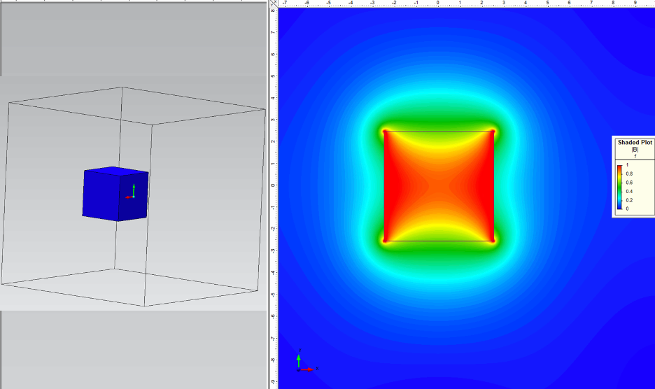
Image 1 – A 3D model of a 5x5x5mm N48 magnet in an airbox (left) and a flux density field map slice cut through the center (right).
For a force analysis, the magnet and the target will need to be specified. The magnetic force between objects will be output as a vector as well, that can be broken down to component directions. Typically, the force will display the overall force on a single object, as it may be acted on by multiple sources. Visualizing the force is much more difficult; it is typically provided as a single value on the target object.
There are a few things to consider when requesting FEA. The simulation will require a lot of input to create the correct environment for the circuit that matches reality. Below is a list of a few of the considerations and a brief explanation:
Software Experience – Simulation software will almost always give you an answer. It likely won’t tell you if something is wrong or if something is inaccurate. It also won’t tell you if you need to factor in surface damage from machining, or small coating or tolerance changes in geometry or material properties. Experience is a large factor in getting a realistic and accurate answer from FEA that can be trusted.
Magnetic Material – to accurately calculate the field in and around the magnet, the material will have to be specified. This is typically in the form of a 2nd quadrant B-H curve, which should be supplied by the magnet manufacturer.
Target Material – for a sensor this might be air or the substrate of the sensor. For a force application, this would be the other magnet or maybe a soft magnetic material (like steel). Soft magnets are typically specified by a 1st quadrant B-H curve. This will provide the software with what is required to calculate the field induced in the target (remember force is a function of the field induced and size).
Temperature – materials act differently at different temperatures. This is especially important for permanent magnet materials as their properties drastically change with temperature. They can also be demagnetized with temperature changes.
Size and Physical Constraints – the size of the magnet and target, as well as any constraints on the size if a certain variable is able to be changed.
Force or Field Targets – a force or flux density target should be specified unless all the sizes and materials are locked.
A solid model for non-basic shapes speeds up analysis (a generic format like STEP or SAT).
Coatings and Geometric Tolerances.
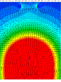
Surrounding Objects – this is especially important if any of the objects near the magnet or target are ferromagnetic. If the objects have a relative permeability that is not VERY close to 1 (that of vacuum) it will affect the results. It is best to think of magnetic analysis as a complete circuit, as one would electrical analysis. Any object around the circuit will change the magnetic field lines and is now part of the circuit. If the object is left out of the circuit, it will induce errors. For an example, see image 2.
Contact Quadrant to gain more magnet insights!